I recently got inspired by the excellent TrumpExcel and his article about dynamic filters but I wanted to update his tool to better suit my needs and reflect the current status of excel (2010+ with tables and references), the concept stays the same but slightly updated.
In my case I had over 1000 internal budget numbers and descriptions, and I wanted a search box to return the IO/Description dynamically to fill a form.
My form was on a different tab than the data and I didn’t want to use to much VBA (I’m more of a formula addict myself whenever I can avoid using VBA)
Concept:
Having a search field that anyone can modify, and output the results of that searchbox to a new table with the matching criteria.
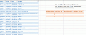
What it will look like in the end:
This gif above (click to expand) shows three use cases: simple search, search with a character wildcard (?), search with a full wildcard (*).
Walkthrough:
Say you have a database (mine was over 1000 lines long as I said)
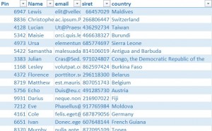
For the exercise’s purpose I created a fake database (thanks to generatedata.com) with PINs, Names, email, SIREN and a country.
Let’s say I want to create a search box to output any data from PIN OR Name OR Country.
Format your data as a table
Alway format your data as a table whenever you want to work on a database (as a general habit).
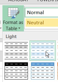
Select all your raw data and go to Home > Format as a Table
Then NAME your table -for that you go to the « Table Tools » tab once you have formated your data as a table, then change the Table Name- (here i named it « database »)
Create a new column grouping all the fields you mean to search
=[@Pin]& » « &[@Name]& » « &[@country]
Here you just create a « helper » column to concatenate all data fields you want to search. You might want that field to be as unique as possible to output all data correctly when you create your search field but that’s not mandatory.
Create a ComboBox for your searchfield
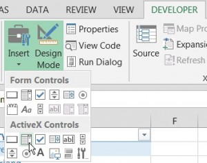
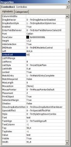
Go to the developer tab in the ribbon and create a ComboBox. Then, right click on the ComboBox you just created and modify its properties.
- Choose « LinkedCell » and input a cell.
This will output anything written in the combobox to the cell you choose. (Here I chose K5) - Style your ComboBox to mimic a searchbox
- Select the cell you linked (K5 in my case) and right clic and « Format Cells », go to the « Protection Tab » and untick « Locked » (this will enable you afterwards to LOCK the entire tab to prevent anyone from touching your precious search box while still having it work properly)

- I generally tend to overlay the ComboBox above the LinkedCell for perfect styling 🙂
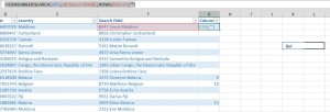
Create a new helper column to search for your data
The idea behind that helper column is to output the row number of the data that matches your search criteria (which you’ll then be able to reuse thanks to an INDEX formula later on… see below)
1 Match your criteria
That’s really the first magic trick and that’s easy enough with the « SEARCH » formula in Excel. (Do use the SEARCH formula and NOT the FIND formula: Search is case INSENSITIVE whereas FIND, on the contrary is case sensitive)
=SEARCH($K$5;[@[Search Field]])
Lock the LinkedCell (hence the $K$5) as your search criteria, and search the first helper column you created (which I called Search Field)
2 Output the row number
Use the ROWS formula combined with an IF and an ISNUMBER formula and the idea is the following (I like to say what my formulas do):
« If, when I search for that search string in my search field I have a number, then it means I found a match, if I found a match, I want the number of that matching row, otherwise, don’t bother me »
=IF(ISNUMBER(SEARCH($K$5;[@[Search Field]]));ROWS($F$2:F2); » »)
There you have to use the ROWS formula (and not the ROW) formula and « hardcode » the reference of your fields (because if the beginning of your table is located elsewhere than on cell A1 -for instance if you work on a table that starts on cell F29 or wherever else).
The ROW formula will return the absolute row number or your row and not the relative position of your row within your table.
Then it’s easy peasy… you « just » have to create your new output.
Create the output fields of your searchbox
Now, we will be using the famous INDEX formula to output the values of your matching search.
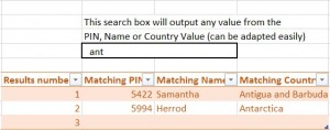
- Define the number of results you want to output and create a table with the number of rows for your results
photo - Use the a combination of INDEX and SMALL functions to output the data:
=INDEX(database[Pin];SMALL(database[search match];[@[Results number]]))
The INDEX formula outputs data on a matching row and column: it works as follow : =INDEX(database;row;column)
- For the column: you can skip the column number if your database only consists of one column right? So on the above formula I input the database[Pin] to reduce my output to only one column (smart right?)
- For the row it’s where the second piece of magic happens: let’s use the SMALL formula as it returns the k’s smallest number in an array of numbers. And to « ask » for the k’s smallest number, just input the « result number » you are looking for (which you just created!)
I personally like to to a bit of cleanup and I add an IFERROR formula to prevent any error from displaying which gives me this final result :
=IFERROR(INDEX(database[Pin];SMALL(database[search match];[@[Results number]])); » »)
Finally I add an IF formula to prevent the output table to display any data if the searchbox is empty and I hide the helper colums:
=IF($K$5= » »; » »;IFERROR(INDEX(database[Pin];SMALL(database[search match];[@[Results number]])); » »))
Et VOILA !
You just need to populate all other fields of your output table to match anything you are searching for.
Do note that the search box will also work with wildcards (* to replace a string and ? to replace a character) making this search field all the more powerful!
You can now protect your sheet and the search box will still work !
Download the Excel Spreadsheet example (I protected the sheet with no password, and note that you can put your database anywhere you want…)
